In this laboratory exercise you will revise basic machine learning concepts and gradient descent optimization and also be introduced to some of the features of Python, numpy and matplotlib. You will implement binary and multinomial logistic regression in Python using numpy You will evaluate your implementation by analysing the quality of classification- This analysis will be done quantitatively (using measures like precision and recall) and qualitatively (by plotting the results using matplotlib). By the end of the exercise you should have revised/acquired the knowledge that will serve as a foundation for the study and development of deep learning models.
During the course of the exercise
you will develop three python modules:
data, binlogreg and logreg.
The data module will contains
methods for creating and plotting
randomly generated 2D data and also
the methods for evaluating classifier performance.
This module will be reused
in the next laboratory exercise
where we will use SVMs
on the same sets of data
to see how it compares to logistic regression.
binlogreg and logreg modules
will contain methods and tests
for binary and multinomial logistic regression.
Understanding derivatives of multivariable vector- and scalar-valued functions is essential for understanding optimization of parameters of a machine learning model using gradient method. A partial derivative of a multivariable function is a derivative of said function with respect to one of those variables while assuming that other variables are constant. A partial derivative of a vector-valued function can be calculated separately for each component of the vector.
Given multivariable vector-valued function f, we demonstrate the process of calculating partial derivatives:
\( \mathbf{f}(\mathbf{x})= \left[ \begin{matrix} x_1^2 + x_2 x_3\\ x_1 + x_2 + x_3\\ \end{matrix} \right] \)
Partial derivative of the first component of \(\mathbf{f}\) with respect to second component of \(\mathbf{x}\) is \( \partial f_1/\partial x_2 = x_3 \) . Partial derivative of the second component of \(\mathbf{f}\) with respect to the first component of \(\mathbf{x}\) is: \( \partial f_2/\partial x_1 = 1 \) .
All of the first-order partial derivatives of a vector-valued function can be expressed using the Jacobian matrix. The rows of the Jacobian correspond to the components of the vector-valued function, while the columns correspond to the components of the independent variable. A Jacobian of a D-variable scalar-valued function has one row and D colums. A Jacobian of a single variable scalar-valued function has one row and one column. A Jacobian of our function \(\mathbf{f}\) has two rows and three columns:
\( \mathbf{f}'(\mathbf{x}) = \frac{d \mathbf{f}}{d \mathbf{x}} = \left[ \begin{matrix} \frac{\partial f_1}{\partial x_1} & \frac{\partial f_1}{\partial x_2} & \frac{\partial f_1}{\partial x_3} \\ \frac{\partial f_2}{\partial x_1} & \frac{\partial f_2}{\partial x_2} & \frac{\partial f_2}{\partial x_3} \end{matrix} \right] = \left[ \begin{matrix} 2x_1 & x_3 & x_2 \\ 1 & 1 & 1 \end{matrix} \right] \)
We will often consider partial derivatives with respect to only some of the independent variables. Going back to our function \(\mathbf{f}\), assuming we are given a vector \(\mathbf{q}\) that contains only the first two components of the vector \(\mathbf{x}\): \(\mathbf{q}=[x_1 x_2]^\top\)), the partial derivative of \(\mathbf{f}\) with respect to \(\mathbf{q}\) can be expressed as:
\( \mathbf{f}'(\mathbf{q}) = \left[ \begin{matrix} \frac{\partial f_1}{\partial x_1} & \frac{\partial f_1}{\partial x_2} \\ \frac{\partial f_2}{\partial x_1} & \frac{\partial f_2}{\partial x_2} \end{matrix} \right] = \left[ \begin{matrix} 2x_1 & x_3 \\ 1 & 1 \end{matrix} \right] \)
Suppose we are given a function \(\mathbf{f}\) which doesn't take the independent variable directly but rather does so indirectly, through another function \(\mathbf{g}\). The resulting function \(\mathbf{F}\) is then the composition of the functions \(\mathbf{f}\) and \(\mathbf{g}\):
\( \mathbf{F}(\mathbf{x}) = ( \mathbf{f} \circ \mathbf{g} ) (\mathbf{x}) = \mathbf{f}( \mathbf{g}(\mathbf{x}) ) \)
We plug-in \(\mathbf{f}\) from the previous section, and assume that function \(\mathbf{g}\) is given as:
\( \mathbf{g}(\mathbf{x}) = \left[ \begin{matrix} \sin(x_1) \\ x_2^3 + x_1 x_2\\ x_3 \end{matrix} \right] \)
We can calculate partial derivatives of \(\mathbf{F}\) with respect to \(\mathbf{x}\)by applying the chain rule for computing partial derivatives. The chain rule is given by the following equation:
\( \mathbf{F}'(\mathbf{x}) = \mathbf{f}'(\mathbf{g}(\mathbf{x})) \cdot \mathbf{g}'(\mathbf{x}) \)
Applying the chain rule to \(\mathbf{F}\) we calculate the Jacobian:
\( \mathbf{F}'(\mathbf{x}) = \mathbf{f}'(\mathbf{g}(\mathbf{x})) \cdot \mathbf{g}'(\mathbf{x}) = \left[ \begin{matrix} 2g_1(\mathbf{x}) & g_3(\mathbf{x}) & g_2(\mathbf{x}) \\ 1 & 1 & 1 \end{matrix} \right] \cdot \left[ \begin{matrix} \cos(x_1) & 0 & 0\\ x_2 & x_1+3x_2^2 & 0\\ 0 & 0 & 1 \end{matrix} \right] \)
\( \mathbf{F}'(\mathbf{x}) = \left[ \begin{matrix} 2\sin(x_1) & x_3 & x_2^3 + x_1 x_2 \\ 1 & 1 & 1 \end{matrix} \right] \cdot \left[ \begin{matrix} \cos(x_1) & 0 & 0\\ x_2 & x_1+3x_2^2 & 0\\ 0 & 0 & 1 \end{matrix} \right] \)
\( \mathbf{F}'(\mathbf{x}) = \left[ \begin{matrix} 2\sin(x_1)\cos(x_1) + x_2 x_3 & x_1 x_3 + 3 x_2^2 x_3 & x_2^3 + x_1 x_2 \\ \cos(x_1) + x_2 & x_1+3x_2^2 & 1 \end{matrix} \right] \)
Properties of multivariable scalar-valued functions are often analysed in machine learning. A typical example would be the loss function that we are trying to optimize (minimize). The gradient of a multivariable scalar-valued function contains partial derivations of the function with respect to all variables. This gradient is usually represented as a column vector, that is to say it is equal to the transpose of a corresponding Jacobian:
\( \nabla f(\mathbf{x}) = \frac{d f(\mathbf{x})}{d \mathbf{x}}^\top \).
We can approximate \(f\) using first order Taylor approximation:
\( f(\mathbf{x} + \Delta \mathbf{x}) = f(\mathbf{x}) + \frac{d f(\mathbf{x})}{d \mathbf{x}} \Delta \mathbf{x} = f(\mathbf{x}) + \nabla f(\mathbf{x})^\top \Delta \mathbf{x} \).
We observe what happens when we change the variable in the direction of the negative gradient:
\(\Delta \mathbf{x} = - \epsilon\cdot \mathbf{g}, \; \mathbf{g}= \nabla f(\mathbf{x}) \).
We see that if the Taylor approximation holds, then displacing the input variable into the direction of the negative gradient should decrease the value of \(f\):
\( f(\mathbf{x} + \epsilon\cdot\mathbf{g}) = f(\mathbf{x}) - \epsilon\cdot \mathbf{g}^\top \mathbf{g} \;. \)
By applying this procedure iteratively, we may arrive to the local minimum of the function \(f\). This is the simplest gradient method and it is called gradient descent. Choosing the right value for \(\epsilon\) is important. The smaller the value of \(\epsilon\), the better the Taylor approximation. However by choosing too small an \(\epsilon\), we risk that our learning algorithm may take too much time. There exist methods that improve gradient descent by optimizing the value of \(\epsilon\). We will review some of them during the lectures.
Multinomial logistic regression is a probabilistic discriminative classification method which models the probabilities of an outcome given input \(\mathbf{x}\). The outcome can be to one of a set of categories \(c_j, j=0, 1, ..., C-1\). It is a generalized linear model that takes an affine transformation of input data and squashes it to the interval [0,1]. We formally model the outcome as a random variable \(Y\) for which we assume the following: \(\sum_j P(Y=c_j|\mathbf{x}) = 1 \; \forall \mathbf{x}\).
In the case of binary logistic regression the number of possible outcomes is 2 (\(C=2\)). The parameters of our model are vector \(\mathbf{w}\) and shift \(b\). The output of the model are a posteriori probabilities of categories \(c_0\) and \(c_1\):
\( P(Y=c_1|\mathbf{x}) = σ(\mathbf{w}^\top\mathbf{x} + b), \mathrm{\ where\ } σ(s)=e^s/(1+e^s) \\ P(Y=c_0|\mathbf{x}) = 1 - P(c_1|\mathbf{x}) \)
Data \(\mathbf{x}\) and vector \(\mathbf{w}\) have the dimensions of Dx1, while \(b\) is a scalar.
In the case of multinomial logistic regression, where the number of possible outcomes is C, we can express their a posteriori probabilities with the following expression:
\( P(Y=c_j|\mathbf{x}) = \mathrm{softmax}(j, \mathbf{W} · \mathbf{x} + \mathbf{b}), j = 0, 1, ..., C-1. \)
In this case, \(\mathbf{W}\) is a matrix with the dimensions CxD and \(\mathbf{b}\) is a vector with the dimensions Cx1. D is the size of input data, while C is the number of classes. We define vector \(\mathbf{s}=\mathbf{W}·\mathbf{x}+\mathbf{b}\) which has a dimension Cx1 and represents classification scores for each possible outcome (category). These scores indicate which outcomes are more/less likely when compared to one another. We can calculate a posteriori probabilities of possible outcomes using softmax function which is defined as: \( \mathrm{softmax}(j, \mathbf{s}) = e^{s_j}/\sum_k e^{s_k} . \)
By furher analysing the softmax function it can be shown that a constant can be added to each classification score without changing the resulting softmax distribution. From the previous fact we can conclude that parameters corresponding to one of the classes can be fixed by assigning them zero value (\(\mathbf{W}_{j,:}=b_{j}=0\) ). The scores can then be interpreted as the likelihood of the rest of the classes with respect to this fixed class. It has been shown to not be necessary in practice as the method for optimising all of the parameters of \(\mathbf{W}\) and \(\mathbf{b}\) converges equally well while keeping the programming code simpler. This redundancy is however useful for stabilizing softmax calculation by preventing numerical overflow when dealing with big exponent. Example of stable softmax calculation:
  # stable softmax
  def stable_softmax(x):
    exp_x_shifted = np.exp(x - np.max(x))
    probs = exp_x_shifted / np.sum(exp_x_shifted)
    return probs
Please note that the above example works only if a first-order tensor (vector) is provided as an input argument. In the exercise, you will need to formulate this procedure for matrix input of the shape \(N\times C\), where each row contains the classification scores of the corresponding data point. Try to achieve this without using an explicit loop.
We can determine the parameters \(\mathbf{W}\) and \(\mathbf{b}\) of logistic regression by optimizing an appropriately defined loss function \(\mathcal{L}(\mathbf{W},\mathbf{b}\) on a training set \(\mathcal{D}\). The training set typically consists of N pairs of inputs and the corresponding outputs: \(\mathcal{D}= \{(\mathbf{x_i},y_i), i = 1, 2, ..., N\}\). For example, if we were classifying 2D data to C categories, \(\mathbf{x_i}\) would be the coordinates of the points on a 2D plane while \(y_i\) would be integers between 0 and C-1. The loss of logistic regression is negative log-likelihood averaged over all training data:
\( \mathcal{L}_\mathrm{NLL} (\mathbf{W},\mathbf{b}|\mathcal{D}) = - \frac{1}{N} \sum_i \log P(Y=y_i|\mathbf{x}_i)\;. \)
Please note that \(P(Y=y_i|\mathbf{x}_i)\) denotes the probability that the datum \(\mathbf{x}_i\) belongs to the labeled class \(y_i\) as predicted by the model. A loss defined this way will favour \(\mathbf{W}\) and \(\mathbf{b}\) that give large probabilities to true outcomes across he training data. Other loss functions could have been used for optimization, but negative log likelihood has been shown to work well and is the most principled solution when dealing with fixed outcomes (eg. true or false).
Unfortunately, some data are not easily associated with with hard labels via one-hot vectors. As an example, we can imagine an image of a brown animal with pointed ears in tall grass. If the annotator is unsure whether it is a cat, a fox, or a dog, the label may be formulated as a distribution where the modes correspond to the likely classes. Negative log-likelihood is not directly applicable in this case, because instead of a correct class index \(y_i\), we now have soft labels that represent categorical distributions over C classes: \(Y_i=[y_{ij}]_{j=1}^C\). Now the loss can be expressed as a weighted average with respect to the soft labels \(Y_i\):
\( \mathcal{L}_\mathrm{CE} (\mathbf{W},\mathbf{b}|\mathcal{D}) = - \frac{1}{N} \sum_i \sum_j y_{ij} \cdot \log P(Y=y_{ij}|\mathbf{x}_i)\;. \)
It turns out that the above expression corresponds to the average cross-entropy (CE) between the true and predicted distribution across all data (verify this as an exercise!).
Note that our equations express the average loss over all observed data. Such formulation simplifies the monitoring of the learning progress and diagnosing issues due to its direct connection with the average prediction accuracy. The initial classification loss on a dataset with 10 classes (CIFAR-10, MNIST) will typically be 2.3 (think about why!). Additionally, the absolute magnitude of the gradients does not depend on the number of data points (i.e., the mini-batch size), which may significantly simplify the tuning of the hyperparameters. For this reason, in practice, we always use the averaged total loss instead of the accumulated total loss.
Optimal parameters of logistic regression (those for which the loss function is minimal) cannot be directly calculated so we usually try to find them using iterative methods. The negative log likelihood loss function \(\mathcal{L}\) is convex, which means that gradient methods such as gradient descent should not get stuck in local extrema. This does not mean that the gradient optimization will work perfectly every time.
Given the loss function \(\mathcal{L}\) we can optimize it using gradient methods. These methods iteratively modify parameters by moving them in the direction of the negative loss gradient. An epoch is the number of iterations after which the training algorithm has seen all of the training data. Number of epoch needed for the algorithm to converge depends on the complexity of the problem we are trying to solve an can be anywhere between a couple to thousands and more.
The main challenge with gradient methods is determining the loss gradient with respect to the model parameter. The loss for the i-th data point can be viewed as a composition of logarithm, softmax and affine transformation of the input. To solve it we will apply the chain rule.
References:
Next we illustrate how to derive the expressions for partial derivatives of the loss function with respect to parameters of binary logistic regression. We define the loss of i-th data pair as \( \mathcal{L}_i(\mathbf{w},\mathbf{b}|\mathcal{x}_i,y_i)= -\log P(Y=y_i|\mathbf{x}_i) \). The partial derivative \(∂\mathcal{L}_i/∂\mathbf{w}\) is a row vector of partial derivatives of the loss \(\mathcal{L}_i\) with respect to elements of \(\mathbf{w}\). Analogously, the partial derivative \(∂\mathcal{L}_i/∂b\) is a row vector of partial derivatives with respect to elements of \(b\).
To make the notation more readable, we define a posteriori probabilities for the i-th class by extending the sigmoid function to include the correct category of input data: \( \sigma_P(y,s)= \begin{cases} \sigma(s),& y=c_1\\ 1-\sigma(s),& y=c_0 \end{cases} = \begin{cases} \frac{e^{s}}{1+e^{s}},& y=c_1\\ \frac{1}{1+e^{s}},& y=c_0 \end{cases} \)
The negative log loss \(\mathcal{L}_i\) can now be expressed as a composition of logarithm function, extended sigmoid function and affine transformation of the i-th data point (remember that \(s_i\) is a scalar that represents the classification score for input \(\mathbf{x}_i\)):
\( \mathcal{L}_i(\mathbf{w},\mathbf{b}| \mathbf{x}_i) = - \log \sigma_P(y_i,s_i)\\ s_i = \mathbf{w}^\top\mathbf{x}_i+ b \)
Using the chain rule, the gradient with respect to model parameters can then be expressed as a product of the Jacobians for \(\mathcal{L}_i\) and \(s_i\):
\( ∂\mathcal{L}_i/∂\mathbf{w} = ∂\mathcal{L}_i/∂s_i · ∂s_i/∂\mathbf{w} \\ ∂\mathcal{L}_i/∂b = ∂\mathcal{L}_i/∂s_i · ∂s_i/∂b \)
Partial derivative of the loss \(\mathcal{L}\) with respect to the classification score \(s\) given input \(\mathbf{x}_i\) is a scalar \(∂\mathcal{L}_i/∂s_i\) which may be regarded as a Jacobian with dimensions 1x1. Partial derivations of classifications score \(s_i\) with respect to parameters \(\mathbf{w}\) and \(b\), are matrices \(∂s_i/∂\mathbf{w}\) with dimensions 1xD and a scalar \(∂s_i/∂b\) that can also be viewed as a Jacobian with dimensions 1x1. Using Iversonovim brackets to denote the influence of the corresponding input category, we can then define the partial derivative of the loss function with respect to the classification score (we assume that \([\![q]\!]\) equals 1 when\(q\) is true and 0 otherwise):
\( ∂\mathcal{L}_i/∂s_i = P(c_1|\mathbf{x}_i) - [\![y_i=c_1]\!] . \)
Partial derivatives of classification scores with respect to model parameters \(\mathbf{w}\) i \(b\) given input \(\mathbf{x}_i\) are:
\( ∂s_i/∂\mathbf{w} = \mathbf{x}_i^\top \\ ∂s_i/∂b = 1 . \)
Using \(\mathbf{g}_s=[∂\mathcal{L}_i/∂s_i]_{i=1}^N\) and taking into account that the total loss is calculated by taking into account the entire training set, the final expressions are:
\( ∂\mathcal{L}/∂\mathbf{w} = 1/N · \sum_i ∂\mathcal{L}_i/∂\mathbf{w} = 1/N · \sum_i g_{si} · \mathbf{x}_i^\top \;,\\ ∂\mathcal{L}/∂b = 1/N · \sum_i ∂\mathcal{L}_i/∂b = 1/N · \sum_i g_{si} \;. \)
To keep the good training performance we will use libraries that have been optimized to perform vector and matrix calculation. We will however consider how to simplify gradient calculation to avoid unnecessary loops.
First we note that partial derivative calculation of \(∂\mathcal{L}/∂\mathbf{w}\) can be represented as a matrix product. We organize input data into a matrix \(\mathbf{X}\) with dimensions NxD. The rows of the matrix \(\mathbf{X}\) correspond to the input data \(\mathbf{x}_i\). We represent the partial derivatives with respect to classification scores as a column vector \(\mathbf{g}_s\) with dimensions 1xN where \(\mathbf{g}_s = [∂\mathcal{L}_i/∂s_i]_{i=1}^N\). The loss gradient with respect to k-th element of \(\mathbf{w}\) can then be represented as a dot product between the vector \(\mathbf{g}_s\) and the k-th column of the matrix \(\mathbf{X}\):
\( ∂\mathcal{L}_i/∂w_k = 1/N · \sum_i g_{si} · x_{ik} = 1/N · \mathbf{g}_s^\top \mathbf{X}_{:k} . \)
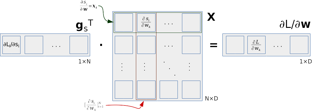
Partial derivatives of the loss function with respect to all elements of \(\mathbf{w}\) can then be represented as a dot product between the vector \(\mathbf{g_s}^\top\) and the data matrix \(\mathbf{X}\):
\( ∂\mathcal{L}/∂\mathbf{w} = \mathbf{g_s}^\top \cdot \mathbf{X} \;. \)
We illustrate this dot product in the following picture. The rows of the data matrix contain individual inputs and represent partial derivatives of corresponding classification scores with respect to \(\mathbf{w}\). The columns of the data matrix correspond to the partial derivative of classification scores with respect to corresponding components of \(\mathbf{w}\). The partial derivative of the loss with respect to the j-th component of \(\mathbf{w}\) is then the result of the dot product of \(\mathbf{g_s}\) and the j-th column of the data matrix \(\mathbf{X}\).
Note two final implementation details.
First, we organized the data within a NxD matrix
in order to ensure that all components of a single data point
are stored at consecutive memory locations.
This means that performing batch operations and mixing data
will result in fewer cache misses.
Second, we will we will need to transpose grad_w
so that its dimensions match the dimensions of \(\mathbf{w}\).
The equations for gradients of negative log loss function with respect to parameters of multinomial logistic regression log very similar to their 'binary' counterparts. This is because the sigmoid function is just a special case of the softmax function. However the representation of the parameter gradients will get complicated due to their specific structure (which in this instance is a matrix). To start, we will look at the gradients for each individual row of the matrix \(\mathbf{W}\), and the corresponding element of the vector \(\mathbf{b}\). The number of these rows/elements is C and we will denote them as \(\mathbf{W}_{j:}\) and \(b_j\). Their partial derivations therefore can be written as \(∂L/∂\mathbf{W}_{j:}\) and \(∂L/∂b_j\) respectively. The gradient of the loss with respect to \(\mathbf{W}_{j:}\) is a matrix with dimensions 1xD, and the gradient of the loss with respect to \(b_j\) is a matrix with dimensions 1x1. Like before, we will use Iverson brackets to denote whether aht input data point belongs to j-th category or not. The equation for the partial derivative of the loss function for the i-th data point \(\mathcal{L}_i\) with respect to the j-th classification score is: \( ∂\mathcal{L}_i/∂s_{ij} = P(Y=c_j|\mathbf{x}_i) - [\![y_i=c_j]\!]. \)
It would be a good idea to derive this formula as an exercise.
We can assemble all of the partial derivatives into a single matrix \( \mathbf{G}_\mathbf{s}= [[∂\mathcal{L}_i/∂s_{ij}]_{j=1}^C]_{i=1}^N \) which has dimensions NxC. To calculate this matrix efficiently, we introduce two auxiliary matrices. The matrix \(\mathbf{P}_{ij} = P(c_j|\mathbf{x_i})\) contains a posteriori probabilities for all datapoints and classes. The matrix \(\mathbf{Y}\) contains the true class for each data point and is defined by the following expression::
\(\mathbf{Y}_{ij}= \begin{cases} 1,& y_i = c_j\\ 0,& y_i \neq c_j \; . \end{cases} \)
This means that we can express the matrix containing partial derivatives of the loss with respect to classification score in the following way: \( \mathbf{G}_\mathbf{s} = \mathbf{P} - \mathbf{Y} \; . \)
The partial derivative of the classification score with respect to parameters of logistic regression look the same as with the binary logistic regression:
\( ∂s_{ij}/∂\mathbf{W}_{j:} = \mathbf{x_i}^\top \\ ∂s_{ij}/∂b_j = 1 . \)
Using the chain rule to get the the gradient of the loss with respect to input parameters and also taking into account the loss across the entire training set, we get the following expressions:
\( ∂\mathcal{L}/∂\mathbf{W}_{j:} = 1/N · \sum_i ∂\mathcal{L}_i/∂\mathbf{W}_{j:} = 1/N · \sum_i ∂\mathcal{L}_i/∂s_{ij} · ∂s_{ij}/∂\mathbf{W}_{j:}\\ ∂\mathcal{L}/∂\mathbf{W}_{j:} = 1/N · \sum_i G_{sij} · \mathbf{x}_i^\top \\ ∂\mathcal{L}/∂b_j = 1/N · \sum_i ∂\mathcal{L}_i/∂b_j = 1/N · \sum_i G_{sij} . \)
Note the similarities with the equations we got for the binary logistic regression. This is because the rows of the matrix \(\mathbf{W}\) affect the loss function in the same way as the vector \(\mathbf{w}\). Analogously, we can calculate the gradient \( ∂\mathcal{L}/∂\mathbf{W}_{j:} \) as a dot product between the j-th column of the matrix \(\mathbf{G}_s\) (denoted as \(\mathbf{G}_{\mathbf{s}:j}\)) and the matrix \(\mathbf{X}\):
\( ∂\mathcal{L}/∂\mathbf{W}_{j:} = \mathbf{G}_{\mathbf{s}:j} \cdot \mathbf{X} \;. \)
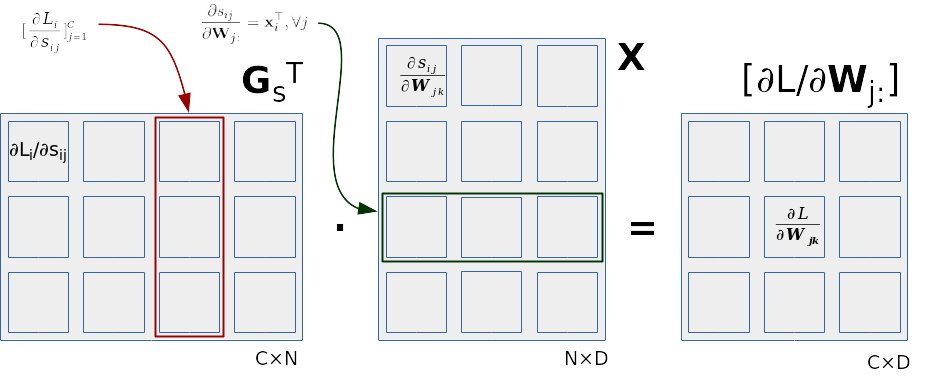
We can improve this further by taking into account that the partial derivative of the j-th classification score with respect to j-th row of the weight matrix are equal for each value of j: \( ∂s_{ij}/∂\mathbf{W}_{j:} = \mathbf{x_i}^\top \forall j . \) Now we can express the gradient of the loss with respect to all rows of the weight matrix with a single matrix product: \( [∂\mathcal{L}/∂\mathbf{W}_{j:}]_{j=1}^C = \mathbf{G_s}^\top \cdot \mathbf{X} \)
This formula is relatively simple to remember but hard to reverse engineer. The most common explanation is that we got to it by simply applying the chain rule. However, that would not be completely true, since we cannot use the simple chain rule to calculate partial derivatives with respect to a matrix argument. If we forced our way along that direction, we would either have to flatten the matrix or accept that the resulting Jacobian would be a third degree tensor. In both cases the complexity of our computations would increase since we would be unable to exploit inherent algebraic structure of our problem which may simply be stated as: \(∂s_{ij}/∂\mathbf{W}_{k:} = 0, j\neq k\). This means you should consider our final expression (\(\mathbf{G_s}^\top\cdot\mathbf{X}\)) as a result of a complicated optimization and not something that will lead you to understand how we derived the expressions for loss gradients. Please take the time to try and understand why it has this form by studying all of the steps we had to take to get it.
We also illustrate how the final matrix product
works in the following figure.
The contribution of the i-th data point
corresponds to the outer product
of the i-th column of \(\mathbf{G_s}^\top\) (shown in red)
and the i-th row of the data matrix (shown in green).
If we took into account only the i-th data point
and considered only the partial derivative
with respect to the weight \(w_{jk}\),
we would only use one element of \(\mathbf{G_s}\),
\(\mathbf{G}_{\mathbf{s}ij}\),
and only the k-th element of the data point
\(\mathbf{x}_i\) in the data matrix \(\mathbf{X}\).
In our implementation, the gradients of the loss with respect to the weights
\(
[\frac{\partial\mathcal{L}}
{\partial\mathbf{W}_{j:}}]_{j=1}^C
\)
will be calculated using only one call
to a library implementing matrix operations, e.g:
grad_W = np.dot(GsT, X).
This solves two problems at once:
np.sum(GsT, axis=1).
We use this approach to avoid loops in high level programming languages, and instead having them in the specialized libraries where they are usually optimized and can be up to 100 times faster than the native c code. More specifically, using numpy compiled using OpenBLAS, dot product implementation is very careful to avoid cache misses and is based on manually optimized machine code for specific architectures. Furthermore, if the OpenBLAS is configured to use OpenMP, our algorithm will make use of all of the processor cores available which shortens the runtime further. You can view some of the performance score here. here. (in these experiments the OpenMP has been used).
Python is a modern dynamic programming language, that has become popular thanks to is applicability to a diverse set of artificial intelligence problems. During this exercise we will be using Python 3. We also recommend using its interactive shell, ipython.
The python code is usually organized into files we refer to as modules. Each module can also contain a short test program which tests its functionality and also shows how the module is meant to be used. We usually put this test at the end of the module within a body of a conditional statement which tests if the module was called as the main program. This way the test is executed each time the module is run.
  if __name__=="__main__":
    # test, test, test!
There are multiple ways to debug Python code. One of the most user friendly types uses Pythons debugger called pdb which can be invoked within the code. First we have to import the pdb module:
import pdb
Then, at the point in the code wher we want to put in our breakpoint we insert the following call:
pdb.set_trace()
This call stops the execution of the program and starts the interactive
shell.
Within the shell you will see all of the data that is available to you when this call was made. you can then print the values of the variables, call other methods and execute other Python operations. You also have some debugging tools available. To see the list of available debugging commands type in help
You will find commands like up,
down and continue useful.
The other way to open the interactive shell from with in the code is by calling
IPython.embed(), but that way you want have the debugging options available.
Finally we show how to generate exceptions using a simple example:
  def proba():
    a=5
    raise ValueError("Iznimka!")

  if __name__=="__main__":
    proba()
By testing this program, we can see that it always ends with a
ValueError exception.
What is a little harder to get is the state of the program when the exception occured (e.g. the value of variable a).
Here we can start the debugger by running
pdb proba.py
and runninig the commandbe continue
(or its shorthand "c").
The debugger runs the program, stops when it gets to an exception
and provides access to the program state in the moment
the exception was raised through a text interface.
E.g. we can then run print a
to view the state of a.
We can also run the program from ipython by calling debug after our interactive call to the programs ends in exception..
Numpy
is a popular Python library for numerical operations. We can refer to numpy as np
in our code if we import it this way:
import numpy as np
Matplotlib
is a library often combined with numpy, and it is used to plot a variety of graphs using Python. Again, we wil use a shorthand plt:
import matplotlib.pyplot as plt
Important advantage of numpy
is that iterative processes
can be represented as matrix operations.
Consider for example an affine transformation of input data,
which is an important step in logistic regression.
Input data can be represented as a matrix X
which has dimensions NxD.
Each row of X is
one data point in D dimensional space.
The transposed weight matrix \(\mathbf{W}^\top\)
can be represented as a numpy matrix
W_t with dimensions DxC.
The bias \(\mathbf{b}^\top\) can be represented
as a numpy vector b_t
with dimensions 1xC.
The affine transformation for the entire training set can be implemented in a single statement
using the numpy support
for matrix multiplication and addition:
H = np.dot(X, W_t) + b_t
Note that the dimensions of addends don't match.
The matrix dot product np.dot(X, W_t)
has the dimensions NxC while b_t
has the dimensions 1xC (N != 1).
The numpy makes the assumption that in this case b_t
should be added to each row of this product.
We note that the i-th row of the data matrix
(\(\mathbf{x}_{i} = \mathbf{X}_{i:}^\top\))
represents i-th data point, which implies
that the i-th row of the resulting matrix H
is the result of the following expression:
\(\mathbf{H}_{i:}^\top =
\mathbf{W}
\cdot
\mathbf{x}_{i}
+
\mathbf{b}
\)).
This means that the result is indeed
the affine transformation of every data point.
We have just seen an example of numpy
automatically broadcasting
the element of lesser dimensionality
to make the expression valid.
Though it might take some time
to get used to this way of thinking,
its advantages are the simplification of code and efficiency.
Feel free to download the solution here: data.py.
In the first exercise we will modify
the data module to include the class Random2DGaussian
which will enable us to sample random 2D data
by using Gaussian random distribution.
The class constructor should create parameters
of a bivariate Gaussian random distribution
(vector μ and matrix Σ).
The methodget_sample(n) should return
n randomly sampled 2D data points
represented as a numpy matrix with dimensions Nx2.
Distribution variance and the allowed range of values should be fixed.
Steps:
minx=0, maxx=10,
miny=0, maxy=10);
and store them as class parameters.
np.random.random_sample).
eigvalx = (np.random.random_sample()*(maxx - minx)/5)**2
np.random.multivariate_normal.
np.random.seed(100)
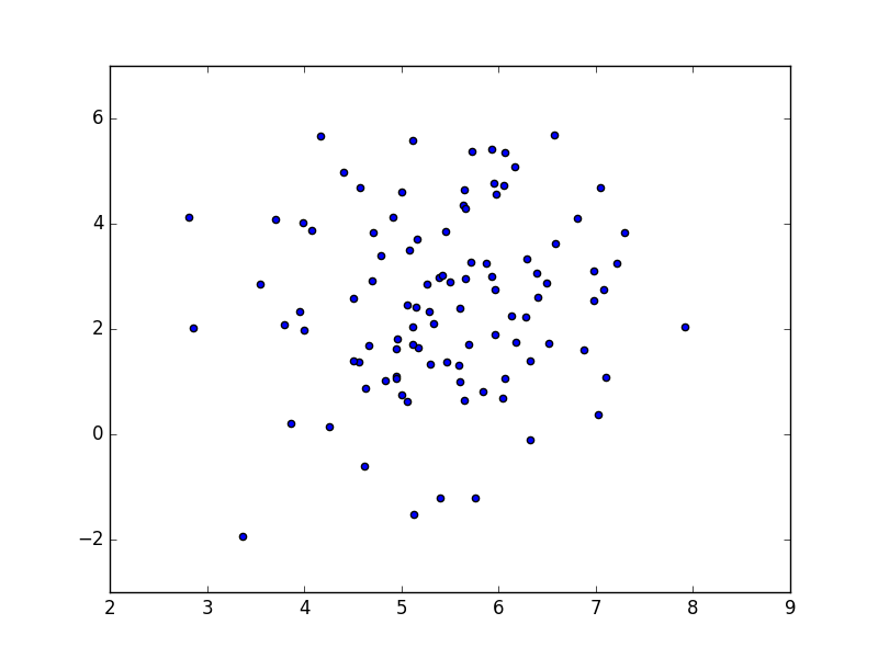
Use the following code to test your implementation:
  if __name__=="__main__":
    G=Random2DGaussian()
    X=G.get_sample(100)
    plt.scatter(X[:,0], X[:,1])
    plt.show()
Depending on the selected seed, your result could look like the one in the following picture:
After you have been satisfied that your code works, store it into data.py.
Implemet a method binlogreg_train
which takes in a training set and learns the parameters
\(\mathbf{w}\) and \(b\) of binary logistic regression. Use the names:
X: the matrix containing the training set, it has the dimensions of NxD
Y_: the vector containing the true classes for the training examples, it has the dimensions Nx1 (to be used during training)
Y: the vector of predicted classes for the training examples, it has the dimensions Nx1 (to be used during evaluation)
Have the function have the following interface:
def binlogreg_train(X,Y_):
  '''
    Arguments
      X:  data, np.array NxD
      Y_: class indices, np.array Nx1

    Return values
      w, b: parameters of binary logistic regression
  '''
Steps:
w using normal distribution N(0,1) (np.random.randn) and have b be 0
param_niter
be a training hyperparameter:
numpy operations
(scores = np.dot(X, w) + b).
numpy operations
numpy operations
grad_w and
grad_b
using numpy operations
w and b
by moving them into the direction of the negative loss gradient,
have param_delta be a training hyperparameter
Here is a sketch of your function:
   # gradient descent (param_niter iteratons)
  for i in range(param_niter):
    # classification scores
    scores = ...    # N x 1

    # a posteriori class probabilities c_1
    probs = ...     # N x 1

    # loss
    loss  = ...     # scalar

    # trace
    if i % 10 == 0:
      print("iteration {}: loss {}".format(i, loss))

    # derivative of the loss funciton with respect to classification scores
    dL_dscores = ...     # N x 1

    # gradijents with respect to parameters
    grad_w = ...     # D x 1
    grad_b = ...     # 1 x 1

    # modifying the parameters
    w += -param_delta * grad_w
    b += -param_delta * grad_b
Implement the function binlogreg_classify
which takes in a set of data points and classifies using logistic regression parameters. Have the function have the following interface:
'''
  Arguments
      X:    data, np.array NxD
      w, b: logistic regression parameters

  Return values
      probs: a posteriori probabilities for c1, dimensions Nx1
'''
Implement the function sample_gauss_2d(C, N)
which creates C Gaussian random distributions, and from each created distribution samples N data points.
The function should return the matrix X
with dimensions (C·N)x2
where the rows correspond to the sampled data points,
and the matrix of true classes Y
with dimensions (C·N)x1
which contains indices of the classes
to which the corresponding points belong.
For example, if the X
was sampled from the Y[i,0]==j.
Implement the function eval_perf_binary(Y,Y_)
which takes in true classes and predicted classes and determines quantitative measures for evaluating classifier performance: accuracy, precision and recall. You can get these values by using the number of true positives (TP), true negatives (TN), false positives (FP) and false negatives (FN).
Implement the function eval_AP which calculates the
average precision
average precision of binary classification. The function takes in an array of true classes \(\mathbf{Y_r}\)
which we get by sorting the matrix of true classes \(\mathbf{Y}\)
using a posteriori probabilities\(P(c_1|\mathbf{x})\).
You can use numpy method argsort for sorting \(\mathbf{Y}\) to get \(\mathbf{Y_r}\).
Average precision is calculated using the following expression:
\(
\operatorname{AP} =
\frac{\sum_{i=0}^{N-1}
\mathrm{Precision}(i) \cdot \mathbf{Y_r}_i}
{\sum_{i=0}^{N-1} \mathbf{Y_r}_i} \; .
\)
\(\mathrm{Precision}(i)\) is the precision you get
if the data with index greater or equal to \(i\)
gets sorted to the class \(c_1\)
and the data with the index less than \(i\) gets sorted into the class \(c_0\).
Your function should have the following behaviour:
>>> import data
>>> data.eval_AP([0,0,0,1,1,1])
1.0
>>> data.eval_AP([0,0,1,0,1,1])
0.9166666666666666
>>> data.eval_AP([0,1,0,1,0,1])
0.7555555555555555
>>> data.eval_AP([1,0,1,0,1,0])
0.5
Write a test for the module binlogreg.py.
You can get your training set using sample_gauss_2d.
After that call the training method and us the return parameters for classifying the training data. Convert the probabilities to get actual class predictions Y (try to do this without using a loop). Evaluate the performance of your classifier using
eval_perf_binary and
eval_AP.
Your code should be like this:
  if __name__=="__main__":
    np.random.seed(100)

    # get the training dataset
    X,Y_ = data.sample_gauss_2d(2, 100)

    # train the model
    w,b = binlogreg_train(X, Y_)

    # evaluate the model on the training dataset
    probs = binlogreg_classify(X, w,b)
    Y = # TODO

    # report performance
    accuracy, recall, precision = data.eval_perf_binary(Y, Y_)
    AP = data.eval_AP(Y_[probs.argsort()])
    print (accuracy, recall, precision, AP)
If you cannot get 100% accuracy, try to find an explanation.
When you are satisfied that your implementation works, store your code into binlogreg.py.
You should put the methods sample_gauss_2d,
eval_AP and eval_perf_binary
into the data.py module.
For those who want to do more:
param_niter,
param_delta
and param_lambda.
Try to find a hyperparameter combination for which your implementation doesn't work. Try to explain why the solution doesn't work with those values.
You can download the solution of this exercise here.
Implement the function graph_data
which is used for visualizing the results
of the binary classification of 2D data points.
Have it implement the following interface:
'''
  X  ... data (np. array Nx2)
  Y_ ... true classes (np.array Nx1)
  Y  ... predicted classes (np.array Nx1)
'''
Steps:
plt.scatter to plot data.
Use named arguments c and
marker to cwspecify
the colour, size and shape of the symbol
used for representing data points
Y_==Y),
and squares for indicating which data points were classified incorrectly.
To avoid using loops in python, you can call plt.scatter twice - once for correctly classified data and one for incorrectly classified data.
Test your code using data sampled from 2 random distributions. For this initial testing you can get predicted classes Y using a dummy classifier e.g.:
  def myDummyDecision(X):
    scores = X[:,0] + X[:,1] - 5
    return scores
Your test could now look something like this:
  if __name__=="__main__":
    np.random.seed(100)

    # get the training dataset
    X,Y_ = data.sample_gauss_2d(2, 100)

    # get the class predictions
    Y = myDummyDecision(X)>0.5

    # graph the data points
    graph_data(X, Y_, Y)

    # show the results
    plt.show()
Here is an example of the possible outcome:
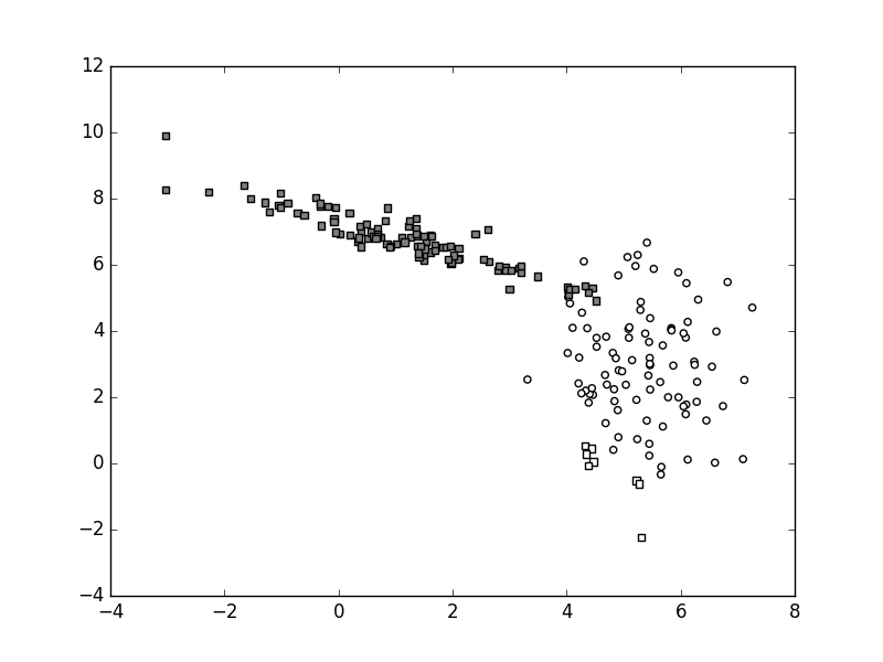
The function myDummyDecision
goes approximately from the upper left corner in the direction of the lower left corner, passing close to the border of the white cluster. This means that most of the data from the white cluster is correctly classified, while all of the gray data is incorrectly classified.
If you are satisfied with the results, store them to data.py.
You can download the solution of this exercise here.
In practice the decision function of a classifier does not return the predicted class for the given data point as was the case with our myDummyDecision. For example, the decision function for the support vector machine returns classification score. The sign of the result determines the predicted class, while the border between the classed is a plane for which every pint has the classification score of zero. The binary logistic regression returns the a posteriori probability \(P(Y=c_1|\mathbf{x})\).
If that probability is greater than 0.5, the classifier classifies the input into \(c_1\).
The border between the classes is a plane/line for which every point has the probability of 0.5. The same interpretation can be given for decision function of deep models, but they can, unlike logistic regression, model non-linear borders between classes. The decision function of these classifiers can be visualised, that is qualitatively evaluated.
That is why we will now implement a way to visualize the decision function. The goal is to implement a methodgraph_surface
which plots the surface of a scalar-valued function of 2D data. We will use this method to plot decision functions of our classifiers which work with 2D data. The interface of graph_surface
should be the following:
'''
  fun    ... the decision function (Nx2)->(Nx1)
  rect   ... he domain in which we plot the data:
             ([x_min,y_min], [x_max,y_max])
  offset ... the value of the decision function
             on the border between the classes;
             we typically have:
             offset = 0.5 for probabilistic models
                (e.g. logistic regression)
             offset = 0 for models which do not squash
                classification scores (e.g. SVM)
  width,height ... rezolucija koordinatne mreže
'''
Similarly to graph_data
we will rely on
matplotlib to visualize the decision function.
To spare the caller from knowing what happens when plotting the function, we will pass the decision function fun
to the method graph_surface
(if you are familiar with design patterns, this is an example of Strategy).
The function fun
takes in the data and returns the predicted class for the given data. This will be wrapper for the classifier whose decision function we want to visualize. To avoid the need for multiple loops, the function should take in a data matrix with dimensions NxD and return a vector containing classification scores with the dimensions Nx1. The rect argument determines the part of the space on for which we are visualizing the decision function. In practice this range depends on the range of our data points: there is no need to visualize the decision plane somewhere where there are no training data.
graph_surface
should also take offset
which determines the value of the decision function on the border between classes. For probabilistic models this value is 0.5, while for models that maximize the margin that value is 0. Finally, graph_surface
should also take the dimensions of the coordinate plane which defines the resolution of the visualization.
Planes are plotted in matplotlib using
np.meshgrid and plt.pcolormesh
(you can see usage examples
here
in official matplotlib
dokumentation).
The procedure is not completely self explanatory so we elaborate more thoroughly:
width×height
within the given rectangle rect
using np.linspace
(or np.arange).
np.meshgrid.
flatten and np.stack
plt.pcolormesh
using reshape.
plt.pcolormesh.
Use the argumens vmin and vmax
to centre the colour palette around the offset
value.
offset.
Use black colour.
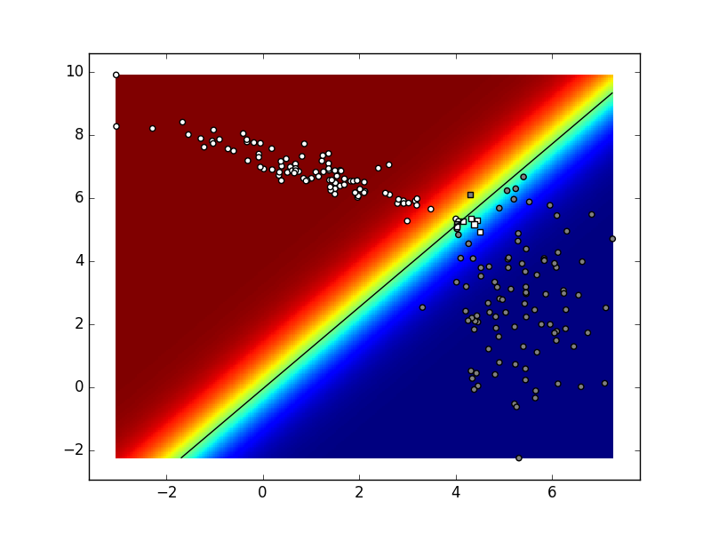
Here is an example of a call to
graph_surface for plotting the decision plane of
myDummyDecision:
    bbox=(np.min(X, axis=0), np.max(X, axis=0))
    graph_surface(myDummyDecision, bbox, offset=0)
If we input this slice of code immediately before calling graph_data in data.py,
we will see the decision plane indicated in rainbow colours, as well as a black line representing the decision border. The white points above the border is white and circular because these points have been correctly classified by
myDummyClassifier,
while the white points below the border are squared because they have been incorrectly classified by
myDummyClassifier.
When you are satisfied with what you have done,
store the code into data.py.
Now we have almost all of the elements needed for fully implementing binary logistic regression. What is left to implement is a function appropriate as a fun argument ofgraph_surface.
In the case of binary logistic regression, this function should take in data matrix X,
and return a vector of a posteriori probabilities for class c1.
The function binlogreg_classify
seems like an appropriate candidate, the only problem being that it has two extra arguments
(w and b).
In programming languaes with static functions this would pose a challenge, however in Python a closure function can be used. A closure function in this case would look like this:
  def binlogreg_decfun(w,b):
    def classify(X):
      return binlogreg_classify(X, w,b)
    return classify
binlogreg_decfun function
returns a local function which remembers the context (w and b). This local function can be used as an argument of graph_surface
(if you are familiar with design patterns, this would be the Decorator pattern. You can achieve the same goal using lambda functions (try to do it as an exercise). If you are a beginner in Python we advise you to start slowly and familiarize yourself with context functions first, befor working with lambda expressions.
The code for the binary logistic regression test would have the following steps:
  # instantiate the dataset
  # ...

  # train the logistic regression model
  # ...

  # evaluate the model on the train set
  # ...

  # recover the predicted classes Y
  # ...

  # evaluate and print performance measures
  # ...

  # graph the decision surface
  decfun = binlogreg_decfun(w,b)
  bbox=(np.min(X, axis=0), np.max(X, axis=0))
  data.graph_surface(decfun, bbox, offset=0.5)

  # graph the data points
  data.graph_data(X, Y_, Y, special=[])

  # show the plot
  plt.show()
Depending on the state of the random number generator and the values of the hyperparameters, the final result for your binary logistic regression classifier could look something like this:
You can even try to make this visualization after every learning iteration and get the following animation. Try to explain the differences in the final state of this animation and the previous picture.
The final task of the first laboratory exercise is to implement logistic regression which can classify data into any number of classes. You need to implement
The gradient descent loop should look something like this:
Implement the function
Implement the function
Implement a decorator for
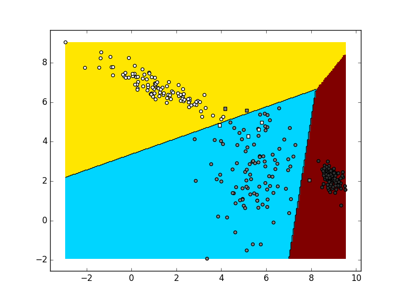
To test your classifier start with only 2 classes. You should get similar results to the binary classifier. After that, try adding one more class and sampling additional data from the third distribution. Take into account that data from each distribution should be marked as belonging to a separate class. Depending on the random generator seed and the values of your hyperparameters, the visualization could be similar to this:
When you are satisfied that your code works, store it into
6. Multinomial logistic regression
logreg_train
that should take in data matrix X
and a matrix of true class indices Y_.
The function returns the logistic regression parameters W and b.
The dimensions of those parameters depend on the number of classes C
which can be determined with the expression max(Y_) + 1.
 # exponentiated classification scores
    # take into account how softmax is calculated
    # in section 4.1 of the text book
    # (Deep Learning, Goodfellow et al)!
    scores = ...    # N x C
    expscores = ... # N x C

    # divisor of the softmax functiona
    sumexp = ...    # N x 1

    # logarithms of aposteriori probabilities
    probs = ...     # N x C
    logprobs = ...  # N x C

    # loss
    loss  = ...     # scalar

    # diagnostic trace
    if i % 10 == 0:
      print("iteration {}: loss {}".format(i, loss))

    # derivative of the loss with respect to scores
    dL_ds = ...     # N x C

    # derivative of the loss with respect to the parameters
    grad_W = ...    # C x D (ili D x C)
    grad_b = ...    # C x 1 (ili 1 x C)
    # modification of the parameters>
    W += -param_delta * grad_W
    b += -param_delta * grad_b
logreg_classify
which returns the matrix of dimensitons NxC
where each row i contains a posteriori probabilities of possible classes \(c_j\), \(j \in \{0, 1, ..., C-1\}\),
for each given data point \(\mathbf{x_i}\).
eval_perf_multi(Y,Y_)
which takes-in indices of true classes and indices of predicted classes and based on that calculates: total classification accuracy, confusion matrix (in which the rows represent the true classes and the columns represent the predicted classes) and vectors of precision and recall for each class.. We recommend first calcualting the confusion matrix which you can then use to calculate other measures.
logreg_classify
which you will pass as an argument tograph_surface.
to visualize what the classifier has trained. There are several ways to visualize the decision function:
logreg.py.
These pages are maintained by Petra Bevandić,
Marin Oršić, Ivan Grubišić, Josip Šarić
and Siniša Šegvić.
The first version of these pages had been created within
the frame of the research project
MULTICLOD
(I-2433-2014) which were funded by Croatian Science Foundation.
The pages have been authored with
vi and
gedit.
Last change: Monday, 21-Apr-2025 15:45:40 CEST
All comments are welcome:

Back