The topic of this exercise are deep models for classification. We'll show that these models can be viewed either as multilayer feedforward neural networks or as augmented logistic regression models which were introduced in exercise zero. Both views lead to the same implementation which iteratively optimizes the likelihood of model parameters. To make development easier and to speed up the experiments, we'll study automatic differentiation opportunities offered by several numeric optimization frameworks. Special attention will be given to Pytorch which is one of the most frequently used tools in this category.
The goal of this exercise is to develop seven modules:
data,
fcann2,
pt_linreg,
pt_logreg,
pt_deep,
ksvm_wrap,
and mnist_shootout.
The module data will be an upgraded
version of the corresponding module from lab 0.
The module fcann2 will contain
the implementation of a two-layer fully-connected model
implemented in terms of Numpy primitives.
This module should be very similar
to the module logreg from lab 0.
Modules
pt_linreg
pt_logreg and
pt_deep
will contain Pytorch implementations
of three machine learning algorithms
with increasing complexity.
The module kswm_wrap will wrap
a kernel-based support vector classifier
based on the module sklearn.svm
from the scikit-learn library,
and enable comparison to the deep classifiers.
Finally, the module mnist_shootout
will evaluate generalization performance
on the MNIST dataset for several
deep learning techniques.
Deep learning models are based on
abstract data representations which we get
by with a sequence of trained nonlinear transformations.
In this and the following laboratory exercises
we consider deep models which are discriminative and
feed-forward.
Discriminative models predict
a conditional probability \(P(Y|\mathbf{x})\)
of a dependent variable \(Y\)
given data \(\mathbf{x}\).
Discriminative models are tipically used when
we have
Artificial neural networks are machine learning models which may be expressed as a directed graph of uniform scalar processing units called artificial neurons. One of the important goals of artificial neural networks is to define a computation model of biological processes. In other words, artifical neurons strive to understand the mechanism of learning in the brains of living organisms. Artificial neural networks are related to deep learning. The main difference is that deep learning does not have an ambition to model biological processes. Instead, the deep learning studies compositional models of practical significance which may not have any biological interpretation.
Artificial neurons tipically conduct an affine reduction of an input vector, which can be concisely expressed as \(f(\mathbf{w}^\top\mathbf{x}+b)\). Here, the vector \(\mathbf{x}\) defines input variables, the vector \(\mathbf{w}\) and scalar \(b\) represent free parameters which are optimized during training, while the non-linear function \(f\) represents the activation of the artificial neuron. The goal of the activation function \(f\) is to introduce non linearity to the model. If we pick a softmax function, the artificial neuron will conduct a multi class logistic regression. If we pick a sigmoid function \(σ(s)=e^s/(1+e^s)\), the artificial neuron will perform binary logistic regression. For better learning of deep models, the sigmoid is being replaced by the rectified linear unit: \(\mathrm{ReLU}(s) = \max(0, s)\).
A neural network with one input layer, softmax on the output, and a loss which maximizes the likelihood of its parameters is equivalent to (possibly multi-class) logistic regression. However, in this course we study deep models which are constructed by adding one or more nonlinear transformations between the input and the output. In the first half of this course, we focus on feed forward models which do not include recurrent connections. Such models can be expressed with acyclic computational graphs where nodes correspond to arbitrary operations, while edges model the connectivity. As in logistic regression, deep feed-forward models are trained by optimizing the likelihood of model parameters given the data and the desired outputs. Contrary to logistic regression, the loss function of deep models is not convex, which means there is no guarantee for finding the global optimum.
In this exercise, we focus on fully-connected feed-forward models. This class of models can be viewed as augmented logistic regression where we introduce several latent layers before the softmax classification. The resulting models are able to achieve nonlinear decision boundaries at a cost of non-convex optimization. Fully-connected feed-forward models can also be viewed as multi-level artificial neural networks. In such networks, neurons can be organized in layers \(S_k\) such that neurons of layer \(k\) operate on all neurons of layer \(k-1\).
We can express each layer of a fully-connected feed-forward model as a composition of an affine vector transform and a nonlinear activation function. For simplicity, we define that applying the scalar transfer function to a vector variable results in elementwise application of the transfer function to the input. Then, we arrive to the following concise notation of the k-th layer of a deep fully-connected feed-forward model with ReLU activation:
\( \mathbf{s_k} = \mathbf{W_k}\cdot\mathbf{h_{k-1}} + \mathbf{b_k} \\ \mathbf{h_k} = \mathrm{ReLU}(\mathbf{s_k}) \)
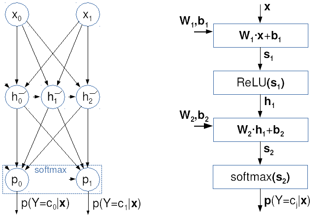
The following illustration displays
two views onto the same
two-layer fully-connected model.
The classic view is shown on the left,
where circles designate
affine scalar neurons and ReLU activations.
The right figure shows a vectorized
computational graph which we use in this course.
Let's consider how to determine the gradients of the negative log-likelihood loss function in the aforementioned example of a two-layer fully-connected model. We'll express the model in vector equations as follows:
\( \mathbf{s_1} = \mathbf{W_1} \cdot \mathbf{x} + \mathbf{b_1} \\ \mathbf{h_1} = \mathrm{ReLU}(\mathbf{s_1}) \\ \mathbf{s_2} = \mathbf{W_2} \cdot \mathbf{h_1} + \mathbf{b_2} \\ P(Y|\mathbf{x}) = \mathrm{softmax}(\mathbf{s_2}) . \)
Our loss function will be the sum of negative log-likelihoods of the model across all data:
\( L(\mathbf{W_1},\mathbf{b_1}, \mathbf{W_2},\mathbf{b_2}| \mathbf{X}, \mathbf{y}) = \sum_i -\log P(Y=y_i|\mathbf{x}_i) \)
We see that the loss function corresponds to a composition of several simpler functions. The loss \(L\) depends on probabilities \(P\) which depend on linear classification scores of the second layer \(\mathbf{s_2}\) which depends on the hidden layer \(\mathbf{h_1}\) and parameters \(\mathbf{W_2}\) and \(\mathbf{b_2}\). The hidden layer \(\mathbf{h_1}\) depends on the linear score \(\mathbf{s_1}\) which finally depends on parameters \(\mathbf{W_1}\) and \(\mathbf{b_1}\) and the data \(\mathbf{x}\). Therefore we determine the gradients of the loss with respect to the parameters using the chain rule.
Partial derivatives of the loss with respect to the j-th rows of \(\mathbf{W_2}\) and \(\mathbf{b_2}\) will be similar to their counterparts in the multiclass logistic regression (cf. lab exercise 0). We'll exploit the algebraic structure of the problem, which can be concisely expressed as: \( \partial {s_2}_{ij}/ \partial \mathbf{W_2}_{k:} = \partial {s_2}_{ij}/ \partial \mathbf{b_2}_{k:} = 0, \; \forall k \neq j \; . \)
In order to achieve a more compact notation we shall denote the k-th row of the matrix \(\mathbf{W_2}\)) as \(\mathbf{W_2}_{k:}\). Furthermore, we express the result in terms of the matrix of a-posteriori probabilities \(\mathbf{P}\) and the matrix of one-hot coded labels \(\mathbf{Y'}\). that we have introduced in lab exercise 0. Finally we get to the following expressions:
\( \frac{∂L_i}{∂\mathbf{W_2}_{j:}} = \frac{∂L_i}{∂{s_2}_{ij}} \cdot \frac{∂{s_2}_{ij}}{∂\mathbf{W_2}_{j:}} = ({P}_{ij} - {Y'}_{ij}) \cdot \mathbf{h_1}_i^\top \; , \\ \frac{∂L_i}{∂b_{2j}} = \frac{∂L_i}{∂\mathbf{s_2}_{ij}} \cdot \frac{∂\mathbf{s_2}_{ij}}{∂b_{2j}} = ({P}_{ij} - {Y'}_{ij}) \; . \)
In order to get the gradient w.r.t. \(\mathbf{W_1}\) and \(\mathbf{b_1}\) we need to propagate over all components of the second layer. However, this propagation is easily expressed because the Jacobian of the linear layer matches the weight matrix, while the Jacobian of the Relu is a diagonal matrix whose diagonal entries reflect the sign of the corresponding component of the first layer. When we arive to the linear score of the first layer, we can reuse much of the work performed in the second layer. In fact, the dependency patterns of the classification score \(\mathbf{s_2}\) w.r.t. the parameters of the second layer is the same as for the linear score \(\mathbf{s_1}\) w.r.t. the first layer parameters. Thus, the analytical expressions of the partial derivatives \(\partial\mathbf{s}_1/\partial\mathbf{W_1}\) are quite similar to the corresponding expressions from the second layer:
\( \frac{∂L_i}{∂\mathbf{s_1}_{i}} = \frac{∂L_i}{∂\mathbf{s_2}_i} \cdot \frac{∂\mathbf{s_2}_i}{∂\mathbf{h_1}_{i}} \cdot \frac{∂\mathbf{h_1}_{i}}{∂\mathbf{s_1}_{i}} \cdot = (\mathbf{P}_{i:} - \mathbf{Y'}_{i:}) \cdot \mathbf{W_2} \cdot \mathrm{diag}([\![s_{1i:}>0]\!]) \;, \\ \frac{∂L_i}{∂\mathbf{W_1}_{j:}} = \frac{∂L_i}{∂{s_1}_{ij}} \frac{∂\mathbf{s_1}_{ij}}{∂\mathbf{W_1}_{j:}} = \frac{∂L_i}{∂{s_1}_{ij}} \mathbf{x_i}^\top \;, \\ \frac{∂L_i}{∂b_{1j}} = \frac{∂L_i}{∂{s_1}_{ij}} \frac{∂\mathbf{s_1}_{ij}}{∂{b_1}_{j}} = \frac{∂L_i}{∂{s_1}_{ij}} \)
In the following text, we shall use the term gradient both for the partial derivation of the loss with respect to the parameters as well as for individual parts of that vector. The exact meaning will be conveyed by the context. The same convention is used in scientific literature. Thus the expression four gradients, refer to the left sides of the above four equations.
It should be noted here that out ambition is not to efficiently calculate some gradients for some data points. On the contrary, our goal is to efficiently calculate all gradients for many data points, by relying on optimized matrix algebra libraries. We follow this strategy since most of speed improvement potential is in cache optimizations which can not be exploited on small data batches. Hence, we will calculate the gradients of each layer for a large batch of data and all parameter rows (as in logistic regression), with a single matrix multiplication.
However, unlike in logistic regression, in deep models we must decide in which order to calculate the particular gradients. (eg should we first calculate \(\frac{∂L_i}{∂\mathbf{b_1}}\) or \(\frac{∂L_i}{∂\mathbf{b_2}}\)). The answer to this ambiguity is provided by the backpropagation algorithm.
Vector equations of our model with two fully connected layers reflect a common theme in deep models: we can see that the partial derivation \(\frac{∂L_i}{∂\mathbf{s_2}_i}\) occurs in gradients of the loss w.r.t all four parameters of the model (\(\mathbf{W_1}, \mathbf{b_1}, \mathbf{W_2}, \mathbf{b_2}\)). This can be used to recover the gradients with minimal computational effort. In fact, we may notice that the gradients of the loss function w.r.t. the nodes of the computational graph do not have to be calculated more than once if they are calculated backwards, from the output towards the input of the model. This simple but very efficient approach is formalized by the backprop algorithm.
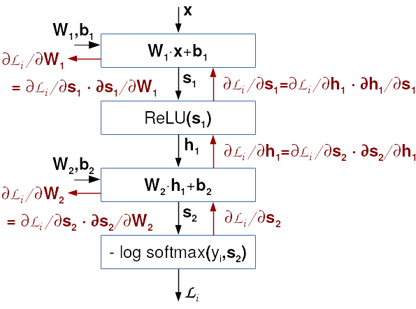
The backprop algorithm is illustrated in the figure below. The black arrows display the evaluation of the model and the loss function of a given data point. This evaluation is called the forward pass. The red arrows show the gradient calculation as suggested by backprop algorithm. This evaluation is called the backward pass.
It appears that all components of the solution to our problem are now known. We know how to calculate gradients w.r.t. certain parameters, as well as the order to do so. However, we wish to emphasize two non trivial details. The first one is the loop through data points. If we would like to enjoy advantages of optimized libraries and avoid iterating in Python, then each gradient should be calculated for a large batch of data at once. If our batch contains N data points,s we'll first calculate the N rows of matrix \( \mathbf{G}_\mathbf{s_2} = [ (\frac{∂L_i}{∂\mathbf{s_2}_{i}})_{i=1}^N ] \), and then 100000 rows of matrix \( \mathbf{G}_\mathbf{h_1} = [ (\frac{∂L_i}{∂\mathbf{h_1}_{i}})_{i=1}^N ] \), etc. Such approach may appear strange, since it heavily increases the memory requirements. However, this is the price for being able to express our algorithms in terms of optimized matrix algorithms. Failing to do so would increase the training by several orders of magnitude.
Another detail is calculating
the gradients of the weight matrices.
Instead of separate calculation of gradients over rows
(as suggested by the equations above),
we advise you to use the approach
from the lab exercise 0
(section 0d).
There we show that the entire matrix of gradients
(which in gradient descent is added to the weight matrix)
can be expressed by a single matrix multiplication.
The weight gradients in the k-th layer
\([\partial L/\partial\mathbf{W_k}]\)
can be obtained for the whole batch at once
by multiplying the transposed gradients
of the linear score
\(\mathbf{G}_\mathbf{s_k}\)
with the input matrix \(\mathbf{H}_{k-1}\).
The vector of gradients for the
k-th layer bias can be calculated
in the similar manner.
However, instead of matrix multiplication
we need to perform column summation
of the matrix \(\mathbf{G}_\mathbf{s_k}\),
which can be obtained by np.sum.
To summarize the discussion for this particular case of a two layer network, we would calculate the partial derivatives of the loss function across all data in the batch in the following order:
In models trained with gradient descent, the initial parameter initialization is highly important. For latent layers activated by the sigmoid function, activations must be centered around zero to allow the sigmoid to be effective. For example, if all inputs were positive, and all weights were positive, all sigmoid activations would be permissive, and the layer's effect would be entirely linear. This is not desirable because a combination of linear transformations is, again, a linear transformation, and we know that linear transformations have much lower capacity than a deep composition of nonlinear transformations. The lesson from this discussion is that deep model learning will progress well if:
PyTorch is an open source library for designing machine learning methods with a special emphasis on the following key functionalities:
Although there are similar other tools (TensorFlow, MXNet, etc.), Pytorch is currently the most popular among researches. It is also suitable for beginers due to its clean architecure and comperhensive documentation.
PyTorch supports various operating systems, but Linux is generally the most well-supported and up-to-date platform for machine learning. For the latest information about PyTorch, you can refer to the official website.
Let's illustrate the design of a program under PyTorch on the following simple example:
import torch
# we define the operation
def f(x, a, b):
    return a*x + b

# we define the variables
# and build a dynamic computational graph
# with a forward pass
a = torch.tensor(5., requires_grad=True)
b = torch.tensor(8., requires_grad=True)
x = torch.tensor(2.)
y = f(x, a, b)
s = a ** 2

# a backward pass that calculates the gradients
# for all tensors that set requires_grad=True
y.backward()
s.backward()               # gradient is accumualted
assert x.grad is None      # pytorch does not calculate gradients with respect to x
assert a.grad == x + 2 * a # dy/da + ds/da
assert b.grad == 1         # dy/db + ds/db

# print out results
print(f"y={y}, g_a={a.grad}, g_b={b.grad}")
The first part of the example defines a regular Python function. The return value of this function will seamlessly fit into PyTorch's computational graph.
The second part of the example creates objects a,
b, and x of type torch.Tensor,
which correspond to nodes in the computational graph.
Tensors a and b have the attribute
requires_grad=True,
which means that PyTorch will compute gradients for them
during automatic backward pass.
Calling operations *, +, and ** creates
new objects of type torch.Tensor,
which are also nodes in the computational graph.
We will refer to objects of type torch.Tensor as tensors.
During the computation of the values of graph nodes, PyTorch remembers all intermediate results that are necessary for gradient computation. The details of this process are determined by the automatic differentiation algorithm (autograd for short).
The third part of the example computes gradients
with respect to the nodes y and x
with the backward method .
Autograd performs backward propagation
all the way back to a and b,
thus computing their gradients.
Multiple calls to the backward method accumulate gradients
in the grad attribute of each tensor declared with requires_grad=True.
It is worth noting that the sequence of calls y.backward(); s.backward()
achieves the same effect as (y + s).backward().
The grad attribute is also
an instance of the torch.Tensor class,
but it is typically separate from the computational graph
that contains its parent tensor.
You can compute higher-order derivatives
by calling the backward method with the argument create_graph=True,
which requests that the derivatives of tensors
are also included in the computational graph.
If you want to recalculate the gradient,
for example, for a different x,
you need to reset the existing gradient to avoid accumulation.
You can achieve this by deleting the grad attribute or
by setting it to None, such as a.grad=None.
If you don't need to compute gradients for a specific computation,
it's a good practice to express it within the torch.no_grad()
context manager, which disables autograd (making PyTorch behave like NumPy).
Here is an example of a procedure that calculates a confusion matrix based
on vectors of true labels y_true and predictions y_pred,
and it returns a confusion matrix of dimensions class_count x class_count.
import torch.nn.functional as F

def multiclass_confusion_matrix(y_true, y_pred, class_count):
  with torch.no_grad():
    y_pred = F.one_hot(y_pred, class_count)
    cm = torch.zeros([class_count] * 2, dtype=torch.int64, device=y_true.device)
    for c in range(class_count):
      cm[c, :] = y_pred[y_true == c, :].sum(0)
    return cm
This example shows that PyTorch enables
the copying of tensors (and computations)
between different platforms/devices using
the optional device argument,
which is accepted by all PyTorch functions
that create new tensors.
Note that you can also specify the data type using
the optional dtype argument.
Instead of the demonstrated torch.zeros function call,
you could specify explicit conversion, like
torch.zeros([class_count] * 2).to(dtype=torch.int64, device=y_true.device),
which would yield the same result but also
leads to unnecessary creation of an intermediate tensor.
Typical values for the device argument are
torch.device('cpu') (the main processor and memory)
or torch.device('cuda:0')
(the first GPU under the CUDA platform).
You can also specify the device as a string:
device='cpu' or device='cuda:0'.
You may find more information in the Pytorch official documentation.
A program that uses PyTorch typically consists of the following components:
torch.nn.Module,
which typically contains other modules with parameters,
Procedures for loading and processing data typically include:
torch.utils.data.Dataset.
__len__ method of this object
typically returns the number of data points.
__getitem__ method of this object
often loads data from the file system
because not all data can fit in memory.
torch.utils.data.Sampler).
torch.utils.data.DataLoader).
The elements of a typical learning algorithm include:
torch.optim.Optimizer.
The following code shows an example of a model which performs an affine transformation:
import torch

class Affine(torch.nn.Module):
  def __init__(self, in_features, out_features):
    super().__init__()
    self.out_features = out_features
    self.linear = torch.nn.Linear(in_features, out_features, bias=False)
    self.bias = torch.nn.Parameter(torch.zeros(out_features))

  def forward(self, input):
    return self.linear(input) + self.bias
The example includes a submodel of type
torch.nn.Linear
(which inherently supports bias, although it's not used in this example)
and a parameter of type torch.nn.Parameter.
The torch.nn.Parameter type is derived from
torch.Tensor and is primarily used
to distinguish parameters from other tensors
(the requires_grad attribute is set
to True by default).
The torch.nn.Module class defines methods
that return iterators over modules(modules),
submodules (children),
parameters (parapeters) etc.
Methods with the prefix named_ return pairs of names (paths)
and objects, as illustrated in the following example.
>>> affine = Affine(3, 4)
>>> print(list(affine.named_parameters()))
[('bias',
  Parameter containing:
  tensor([0.000, 0.000, 0.000], requires_grad=True)),
 ('linear.weight',
  Parameter containing:
  tensor([[-0.2684,  0.2126, -0.4430],
          [ 0.3446, -0.2018, -0.4346],
          [-0.4756, -0.3453,  0.1401],
          [ 0.3257,  0.0911, -0.1267]], requires_grad=True))]
We typically design modules to operate on
mini-batches of data. For example, a call
like affine(torch.randn(5, 3))
results in a tensor of dimensions (5, 4),
where torch.randn(5, 3) creates a matrix
of elements that were randomly from a normal distribution.
More information about modules can be found
in the official documentation.
Various procedures for parameter initialization
can be found in the torch.nn.init package.
The next example demonstrates the basics of data loading:
import numpy as np
import torch
from torch.utils.data import DataLoader

dataset = [(torch.randn(4, 4), torch.randint(5, size=())) for _ in range(25)]
dataset = [(x.numpy(), y.numpy()) for x, y in dataset]
loader = DataLoader(dataset, batch_size=8, shuffle=False,
                    num_workers=0, collate_fn=None, drop_last=False)
for x, y in loader:
  print(x.shape, y.shape)
The example first generates a random dataset of 25 random pairs of 4x4 matrices and scalars. For illustrative purposes, the data is converted to the numpy.ndarray type without copying. The dataset is then passed to the constructor of the DataLoader class, whose instance facilitates iteration over mini-batches.
Here are some important arguments that the constructor accepts:
batch_size argument sets
the size of each mini-batch.
shuffle argument is
a Boolean value that determines whether
a random order should be chosen before
each pass through the data.
num_workers argument
specifies the number of parallel processes for data loading.
collate_fn argument is
a function that organizes individual data points
into mini-batches.
By default, when collate_fn=None,
the torch.as_tensor function is called,
which converts the NumPy array into a torch.Tensor without copying.
drop_last argument is
a Boolean value that determines
whether the last mini-batch
should be dropped if there are
fewer than batch_size elements
remaining for the last mini-batch.
In the example provided, the program will print
torch.Size([8, 4, 4]) torch.Size([8]) three times
and torch.Size([1, 4, 4]) torch.Size([1]) once.
You can find more information about data loading
in the official documentation.
The following procedure describes an example of iteration in supervised learning:
def supervised_training_step(ctx, x, y):
  ctx.model.train()  # model is set into training mode
  output = ctx.model(x)  # forward pass
  loss = ctx.loss(output, y).mean()  # calculate loss

  ctx.optimizer.zero_grad()  # set gradients to 0
  loss.backward()  # backward pass
  ctx.optimizer.step()  # optimization step
ctx is an access object
that encompasses the model model,
the loss function loss,
and the optimization algorithm optimizer.
x and y are
input and output mini-batches.
First, the model is set to training mode because
it may contain modules like dropout or
batch normalization that behave differently
during training compared to evaluation.
Then, in the forward pass,
the model computes the output,
and the loss is calculated for the mini-batch.
Afterward, the optimization step is performed.
The optimizer object is of a type
derived from torch.optim.Optimizer and
references the parameters for optimization.
Here's a simple example of creating an optimizer:
from torch.optim import SGD
optimizer = SGD(model.parameters(), lr=1e-2, weight_decay=1e-4)
The basic arguments are the parameters
and the learning rate lr.
For efficiency, PyTorch offers the option
to apply L2 regularization directly
in the optimizer. This is why you see
the weight_decay argument in the constructor.
The main methods of an optimizer are zero_grad and step.
You should call the zero_grad method
before computing gradients if you don't want them to accumulate.
The step method performs an optimization step.
In the case of gradient descent,
this method updates all parameters by
subtracting their respective gradients scaled by the step size.
For more information about optimizers, you can refer to the official documentation.
You may find the solutions to exercise 1 here.
In our experiments in lab 0, logistic regression achieved quite good classification results. This should not be viewed as a surprise since the sigmoid of affine transformed data was a good fit for the chosen posterior probability of data classes. Our experiments slightly digressed from ideal theoretical assumptions (our classes had different covariances) but results showed that this digression did not hurt the performance of our algorithm. Now we will make the things a little harder by instantiating the data with a more complex generative model.
Instructions:
sample_gmm_2d(K, C, N)
which creates K ≥ C random
bivariate Gaussian distributions,
and samples N data points from each of them.
Unlike in sample_gauss_2d,
here we need to assign class c_i
to each bivariate distribution G_i,
where c_i is randomly sampled
from the set {0, 1, ..., C-1}.
This way we get the data generated by mixtures
of randomly chosen Gaussian distributions.
The function should return a data matrix X
and the groundtruth class matrix Y.
The rows of both matrices
correspond to sampled data points.
The matrix X contains the data,
while Y has on column and
contains the class index
of the generating distribution.
0 to C - 1.
Then, it must sample the required number of data points
from each of the distributions and assign these
data the corresponding class index.
'''
  X  ... data in a matrix [K·N x 2 ]
  Y_ ... class indices of data [K·N]
'''
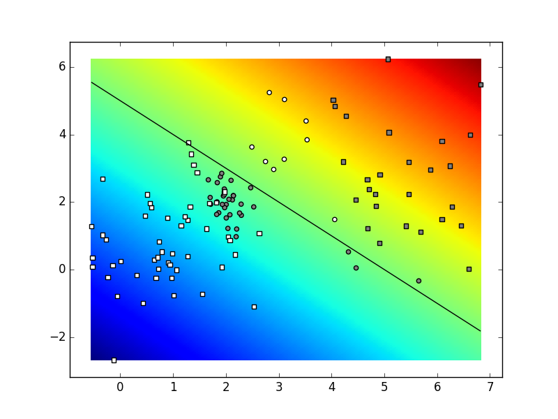
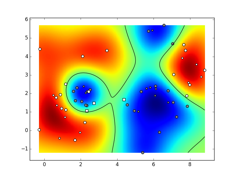
Run the subroutine sample_gmm_2d
and test it by invoking drawing functions
developed in lab exercise 0
(graph_surface and graph_data).
Depending on the parameters and
the state of the random number generator,
your result could look similar to the figure below.
Our parameters were:
K=4,
C=2,
N=30.
When you are satisfied with the execution results,
save the code in the file data.py.
In this exercise you shall develop an algorithm
for learning a probabilistic classification model
with one hidden layer,
by employing the negative log-likelihood loss
and stochastic gradient descent.
Your algorithm should be stored
in the module fcann2.
The organization of the module should follow
the example set by the module logreg
from the lab exercise 0.
The module should contain the methods
fcann2_train
and fcann2_classify.
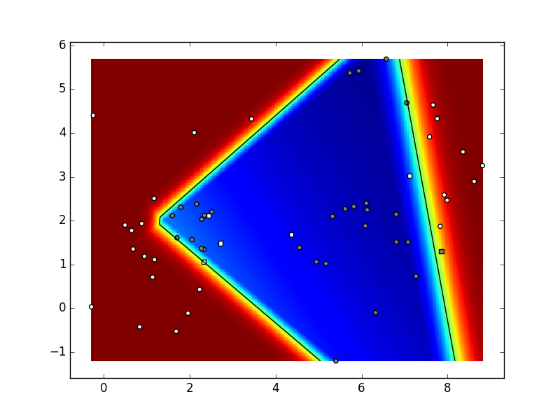
The module should be tested
on an artificial dataset
containing 2D data of two classes sampled
from a Gaussian mixtures of 6 components.
Depending on parameters and the seed
of the random number generator,
your result could look like in the figure below.
Our hyper-parameters were:
K=6,
C=2,
N=10,
param_niter=1e5,
param_delta=0.05,
param_lambda=1e-3 (regularization coefficient),
hidden layer dimensionality: 5.
When you are satisfied with the execution results,
save the code in the file fcann2.py.
We illustrate a typical structure
of a machine learning algorithm in PyTorch
on a complete example of the optimization procedure
for estimating the parameters of a line
y = a * x + b
passing through points
(1,3) and (2,5).
import torch
import torch.nn as nn
import torch.optim as optim


## Defining the computational graph
# data and parameters, parameter initialization
a = torch.randn(1, requires_grad=True)
b = torch.randn(1, requires_grad=True)

X = torch.tensor([1, 2])
Y = torch.tensor([3, 5])

# optimization procedure: gradient descent
optimizer = optim.SGD([a, b], lr=0.1)

for i in range(100):
    # affine regression model
    Y_ = a*X + b

    diff = (Y-Y_)

    # quadratic loss
    loss = torch.sum(diff**2)

    # gradient calculation
    loss.backward()

    # optimization step
    optimizer.step()

    # setting gradients to zero
    optimizer.zero_grad()

    print(f'step: {i}, loss:{loss}, Y_:{Y_}, a:{a}, b {b}')
Assignments:
a and b.
Define the nodes which calculate
the gradients explicitly.
Print out values of the gradients and make sure
they are equal to the values determined by PyTorch.
When you are satisfied with the execution results,
save the code in the file pt_linreg.py.
In this assignment we shall implement logistic regression with Pytorch. The source code will be only half as long as the corresponding "hand made" code from the lab 0. The exercise will demonstrate the following PyTorch advantages: i) we don't need to derive gradients, and ii) the code may be executed on different processing platforms (CPU, GPU) without making any changes to the code. These advantages will be crucial in cases of large models with hundres of millions of parameters (in smaller models, a CPU implementation may be faster due to expensive transfers from RAM to GPU).
In PyTorch, you typically define a model
by inheriting from the base class torch.nn.Module.
In doing so, you need to define a constructor
(__init__) and a forward function,
which represents the forward pass through the model.
You express model parameters as attributes
of type torch.nn.Parameter.
This allows you to easily access model parameters
using torch.nn.Module.parameters().
Here's an example of what a logistic regression
learning module could look like:
class PTLogreg(nn.Module):
  def __init__(self, D, C):
    """Arguments:
       - D: dimensions of each datapoint
       - C: number of classes
    """

    # parameter initialization (use nn.Parameter):
    # potential names: self.W, self.b
    # ...

  def forward(self, X):
    # forward pass through the model: calculate probabilites
    # use: torch.mm, torch.softmax
    # ...

  def get_loss(self, X, Yoh_):
    # loss formulation
    # use: torch.log, torch.exp, torch.sum
    # be mundful of numerical overflow and underflow
    # ...


def train(model, X, Yoh_, param_niter, param_delta):
  """Arguments:
     - X: model inputs [NxD], type: torch.Tensor
     - Yoh_: ground truth [NxC], type: torch.Tensor
     - param_niter: number of training iterations
     - param_delta: learning rate
  """

  # optimizer initialization
  # ...

  # training loop
  # print out loss values during training
  # ...


def eval(model, X):
  """Arguments:
     - model: type: PTLogreg
     - X: actual datapoints [NxD], type: np.array
     Returns: predicted class probabilites [NxC], type: np.array
  """
  # you need to transform the input into torch.Tensor
  # you need to transform outputs into numpy.array
  # use torch.Tensor.detach() and torch.Tensor.numpy()
Notice that unlike the previous exercise
the true labels of the training data
are now called Yoh_
instead of Y_.
This is due to the fact that
the cross entropy loss is more easily expressed by
organizing the labels in a matrix
n which the rows correspond to data points
while the columns correspond to class labels
(this is also known as one-hot notation).
If a data point x_i
matches the class c_j,
then Yoh_[i,j]=1 and
Yoh_[i,k]=0 for all
k!=j ("one hot").
In former mathematical discussion,
data labels organized in such manner
were referenced by the matrix \(\mathbf{Y'}\).
The structure of a test program should be very similar to the test programs from the previous exercise:
if __name__ == "__main__":
  # initialize random number generator
  np.random.seed(100)

  # define input data X and labels Yoh_

  # define the model:
  ptlr = PTLogreg(X.shape[1], Yoh_.shape[1])

  # learn the parameters (X and Yoh_ have to be of type torch.Tensor):
  train(ptlr, X, Yoh_, 1000, 0.5)

  # get probabilites on training data
  probs = eval(ptlr, X)

  # print out the performance metric (precision and recall per class)

  # visualize the results, decicion surface
Assignments:
PTLogreg
and check whether your program
achieves the same results
as the corresponding programs from lab 0 for
two or three classes. You should formulate
the loss so that it does not depent on the
size of the training data (this makes it easier to
interpret the loss value and validate the
learning step).
param_lambda.
Test the effect of regularization to the shape
of the prediction surface.
When you are satisfied with the execution results,
save the code in the file pt_logreg.py.
Our next task is to expand
the Tensorflow implementation of logistic regression
in a way to enable simple creation of
configurable fully connected classification models.
Our new class will be named PTDeep
and should have a similar interface
to the class PTLogreg.
The PTDeep constructor will recieve an aditional
configuration hyperparameter
in the form of a list of layer dimensionalities.
Additionaly, the constructor will recieve the activation function
of the hidden layers.
The element at index 0 defines
the dimensionality of the data.
Elements at indices 1
to n-2 (if any)
define the number of activations in hidden layers.
The last number in the configuration list
(the element at index n-1)
corresponds to the number of classes
(the model is supposed to perform the classification).
For example, a configuration [2,3]
gives rise to multi-class logistic regression
of two dimensional data into three classes.
The configuration [2,5,3] specifies
a model with one hidden layer h
which contains 5 activations:
h = f (X * W_1 + b_1)
  probs = softmax(h * W_2 + b_2)
  X     ... [?,2]
  W_1   ... [2,5]
  b_1   ... [1,5]
  h_1   ... [?,5]
  W_2   ... [5,3]
  b_2   ... [1,3]
  probs ... [?,3]
Implementation of the class PTDeep
should be very similar to what we had for
the PTLogreg class.
In the constructor, you need to initialize
weight matrices and bias vectors.
Since the number of layers can vary,
you'll need to store weight matrices
and bias vectors in lists
(let's call them self.weights and
self.biases).
To fully leverage the capabilities of
the torch.nn.Module superclass,
the attribute representing the list of parameters
should be of type torch.nn.ParameterList,
and its members should be of type torch.nn.Parameter.
Non-linearity in hidden layers can be expressed
using functions like torch.relu,
torch.sigmoid, or torch.tanh.
Assignments:
PTDeep
and try out configuration [2,3]
on the same data as in the former assignment
(the test code should be very similar).
Make sure the results are the same as before.
count_params method
that will print the symbolic name
and dimensions of all parameters' tensors.
Additionally, the function should calculate
the total number of model parameters
(e.g., for the configuration [2, 3],
the result should be 9).
We can now use the named_parameters
iterator elegantly to traverse all model parameters.
data.sample_gmm_2d(4, 2, 40) and
data.sample_gmm_2d(6, 2, 10),
using configurations [2,2], [2,10,2] and [2,10,10,2].
Print accuracy, recall, precision
and average precision.
Display the classification results
and observe the decision surface.
If there is no convergence,
consider changing the hyperparameters.
Based on parameters and the state
of the random number generator,
your result could be similar
to the animation below
(our hyperparameters were:
K=6,
C=2,
N=10,
param_niter=1e4,
param_delta=0.1,
param_lambda=1e-4
(regularization coefficient),
config=[2,10,10,2], ReLU).
When you are satisfied with the execution results,
save the code in the file pt_deep.py.
Recall the properties of the kernel SVM
(model, loss, optimization)
and read the documentation od the module svm
from the library scikit-learn.
Design the class KSVMWrap
as a thin wrapper around
the module sklearn.svm
which you are going to be apply to
the same two-dimensional data as before.
Considering the spmlicity of our wrapper,
the training can be done from the constructor,
while class predictions, classification scores
(required for average precision) and support vectors
can be fetched in methods.
Make the interface of the class as follows:
'''
Metode:
  __init__(self, X, Y_, param_svm_c=1, param_svm_gamma='auto'):
    Constructs the wrapper and trains the RBF SVM classifier
    X,Y_:            data and indices of correct data classes
    param_svm_c:     relative contribution of the data cost
    param_svm_gamma:  RBF kernel width

  predict(self, X):
    Predicts and returns the class indices of data X

  get_scores(self, X):
    Returns the classification scores of the data
    (you will need this to calculate average precision).

  suport:
    Indices of data chosen as support vectors
'''
Assignments:
data.graph.data
by introducing the argument special.
The argument special
assigns a list of data indices
which are to be emphasized by
doubling the size of their symbols.
TFDeep and KSVMWrap
on a larger number of random data sets.
What are the pros and cons of their loss functions?
Which of the two guarantees a better performance?
Which of the two can take a larger number of parameters?
Which of the two would be more suitable for
2D data sampled from Gaussian mixtures?
special
of the function data.graph.data
to emphasize the display of support vectors.
Based on the parameters and the random number generator,
your results could resemble the following animation.
(our hyperparameters were:
K=6,
C=2,
N=10,
param_svm_c=1,
param_svm_gamma='auto').
When you are satisfied with the execution results,
save the code in the file ksvm_wrap.py.
So far, the trained models haven't been evaluated on a separate test set. Such experiments can not provide an estimate of the generalization performance. They are therefore appropriate only in early experiments where we test whether a model has enough capacity for the given task.
In this exercise we shall explore generalization performance on real data. The MNIST dataset is a collection of hand-written images of digits from 0 to 9. Each digit is represented by an image of 28x28 pixels. MNIST contains 50000 training images and 10000 testing images. The dataset can be (down)loaded with the following code:
import torch
import torchvision

dataset_root = '/tmp/mnist'  # change this to your preference
mnist_train = torchvision.datasets.MNIST(dataset_root, train=True, download=True)
mnist_test = torchvision.datasets.MNIST(dataset_root, train=False, download=True)

x_train, y_train = mnist_train.data, mnist_train.targets
x_test, y_test = mnist_test.data, mnist_test.targets
x_train, x_test = x_train.float().div_(255.0), x_test.float().div_(255.0)
This approach for acquiring the MNIST dataset may sometimes encounter a 503 error. If that happens, we suggest the following alternative procedure:
Now, the sets of images and class indices
are represented by PyTorch tensors
x_train,
y_train,
x_test and
y_test.
We can find the dimension of the data by
querying the shape of those matrices.
N=x_train.shape[0]
D=x_train.shape[1]*x_train.shape[2]
C=y_train.max().add_(1).item()
We may display input images with plt.imshow function.
We recommmend you use cmap = plt.get_cmap('gray').
Assignments:
PTDeep model
with configuration [784,10] on MNIST.
Plot and comment on the weight matrices
for each digit separately. Repeat this
for different regularization values.
n mini-batches.
Then perform one training step
for each mini-batch.
Store the code into the train_mb method.
Estimate the effect of the convergence quality
and achieved performance
for the most successful configuration
of the previous assignment.
In order to properly coprehent batch learning,
you are not allowed to use
torch.utils.data.DataLoader
torch.optim.Adam
with fixed learning rate of 1e-4.
Estimate the effect of this change to
the quality of convergene and achieved performance.
torch.optim.lr_scheduler.ExponentialLR.
This function should be called after each
epoch as is recommended in the documentation
Leave the initial learning rate as before,
and change the other hyperparameters to
gamma=1-1e-4.
sklearn.svm.
Use the one vs one SVM variant
to allow the classification of multiclass data.
The experiment might require some patience
since the training and evaluation may takes
up to more than half an hour.
Compare the achieved performance
with the performance of deep models.
When you are satisfied with the execution results,
save the code in the file mnist_shootout.py.
Study the batch normalization technique for fully connected models. Expand the deep classifier in exercise 5 by fitting a batchnorm layer after the affine transformations in each hidden layer. Be careful to allow the change of batch-normalization parameters only during training. Compare the performance to what you have obtained with the basic deep model. Consider problems that can arise while training models with normalization layers.
|
These pages are maintained by Petra Bevandić,
Marin Oršić, Ivan Grubišić, Josip Šarić
and Siniša Šegvić.
The first version of these pages had been created within the frame of the research project MULTICLOD (I-2433-2014) which were funded by Croatian Science Foundation. The pages have been authored with vi and gedit. Last change: Friday, 04-Apr-2025 12:49:11 CEST | |
All comments are welcome:

| Back |